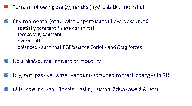
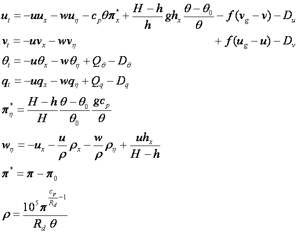
The numerical model presented here is similar to many other mesomodels. The model equations are based on the atmospheric primitive equations in a terrain-following coordinate system and simplified by adoption of the anelastic and Boussinesq approximations. (similar to eg,  Zdunkowski and Bott 2003, CUMM of Huang 2000, Sha et al 1996 and Finkele 1995). After transformation from the usual Cartesian coordinates (x, y, z) to the terrain-following coordinate (x, y, η) with

 

 

 

where h(x, y) is the height of the topography and H is the height of model domain, the governing equations of the three-dimensional, hydrostatic and anelastic, and dry numerical model are

 

 

 

 

 

 

 

 

 

 

 

 

 

 

 

 

 

 

 

 

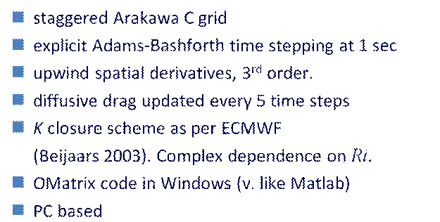
where p is the scaled pressure (the Exner function).  Variables subscripted with “0” such as, p₀ and θ₀ ,are the mesoscale deviations of pressure and potential temperature from the basic state. Besides the usual symbols in the aforementioned equations Q represents the net source/sink term for the scalar variable concerned and D represents vertical and horizontal diffusive drag for the variable concerned.

In the turbulence modeling, the vertical turbulent eddy diffusivity K-closure scheme is used (for detail see eg, Beijaars A, 2003; Turbulence and Mixing in Parameterization of Physical Processes in ENCYCLOPEDIA OF OCEAN SCIENCES Elsevier Press, pp1710-1712).

The horizontal eddy diffusivity for momentum K_hm in a nonlinear three-dimensional form defined as

 

 

was used, where β ~ 0.05 is a constant.

 

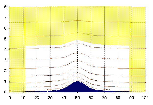
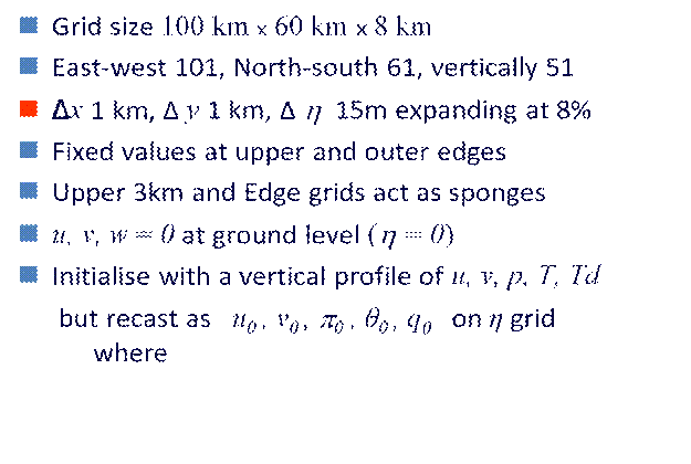
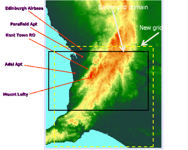
a. Numerical aspects and computational domain

In the horizontal directions, a grid interval of Δx = Δy = 1000 m is adopted, while in the vertical direction an expanding grid, with the greater resolution ΔZ = 15 m near the ground, is used. The domain of 110km by 110km with the top boundary is located at z = 8.6 km comprising of  111 by 111 by 51 grid points. The prognostic equations are integrated forward explicitly in time using third order Adams-Bashforth scheme with the time step chosen to satisfy the CFL criterion, generally 1 sec.  Third order upwind differences are used in horizontal space; weighted second order differencing is used in the vertical. To increase the accuracy and stability of the finite difference approximations, a staggered grid is used, both horizontally and vertically.

b. Boundary and initial conditions

A no-slip lower boundary condition u = = w = 0 is imposed. The surface temperature is constant and set at the air temperature of the initial column for corresponding altitudes. At the upper boundary all variables are fixed at their initial values. In the upper levels of the model, about half the vertical domain, an absorbing layer is employed using Rayleigh damping to suppress downward reflection of energy. At all lateral boundaries, all variables are fixed at their initial values, with an absorbing region similar to that in the upper level installed over the 10 grid points adjacent to the boundaries. This serves to maintain the integrity of the upstream profiles throughout the integration and to prevent spurious wave reflection at the outflow boundaries.  The linear vertical profile of potential temperature and uniform profile of velocity are used to initialize the model by assuming the profiles horizontally homogeneous in the computational domain. The initial flow is assumed to be in geostrophic balance but within the friction layer (~ 400m) an Ekman-gradient is evolved by running the model without topography to quasi-steadystate. Monin–Obukhov similarity law is used to determine the surface heat and momentum fluxes and u, , and θ at the nearest grids above the lower boundary.

The potential temperature and the Exner function  are divided in to mean fields and perturbation fields. The mean fields are assumed to be in geostrophic and hydrostatic balance – except in the friction layer where a diffusion-coriolis balance (Ekman layer) is assumed.

 

BACK