Fitting
a Binormal Distribution to Daily Temperatures
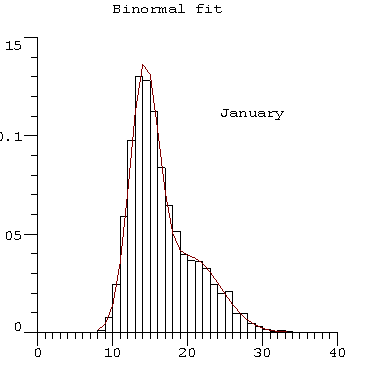
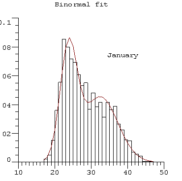
Shown are examples of comparisons of actual distribution functions compared binormal (in red) for the South
Australian capital city of
Maximum temperatures also in January.
A binormal population is composed of two subpopulations each of which is normal or Gaussian.
So the pfd is defined as -
Pfd=
weight1*N(mean1, sigma1) + weight2*N(mean2,
sigma2).
where N denotes the Gaussian. Grace and Curran (1993) showed the applicability of this concept to the daily maximum temperature at several stations in southern Australia.
A reiterative procedure is used to find the six unknowns above. Test statistics such as Kolmogorov and Cramer-Von
Mises reject a hypothesised single normal distribution,
but accept the binormal. This is true for any month. It is also true for most
locations in
The tails of the red binormal distribution fit the observed distribution quite well especially at the tails and clearly fit
much better than would a single normal. Often, a knowledge of the true likelihood of the occurrence of extremes is very
important. One such application is to provide a reliable determination of probabilities of frost occurrence.


Horizontal axes show minimum and maximum temperatures (in °C
at
occurrence as a relative fraction.
OMatrix scientific
programming package is suitable and easy-to-use software to accomplish the
fitting on the daily temperature datasets kindly supplied by the Australian Bureau
of Meteorology.
GRACE, W.J. and CURRAN, E.F. 1993. A Binormal Model of
Frequency Distributions of Daily Maximum Temperature. Aust.
Met. Mag. 42, 151-161.